Apache Iceberg 101 to Deep dive — From Theory to Hands-ons with Docker

Iceberg from Theory to Architecture and setup with Pyspark 3.5.x version with Docker and Iceberg. It helps guys having a quick look how Apache Iceberg works and provides a ready environment to hand-on

Jun 01, 2025

Start writing today. Use the button below to create a Substack of your own

Modern data lakes increasingly demand the reliability of databases and the scalability of big data platforms. Enter Apache Iceberg, an open table format that brings SQL table simplicity to petabyte-scale data. Iceberg was originally developed at Netflix to overcome limitations of Hive tables (which lacked ACID guarantees) and was open-sourced via the Apache Software Foundation in 2018. It has since emerged as a critical component in data lakehouse architectures, enabling multiple engines (Spark, Trino, Flink, etc.) to safely work on the same data at the same time.

What is Apache Iceberg? In a nutshell, Iceberg is a high-performance table format for huge analytic datasets (from Apache Iceberg). Instead of querying raw files (like Parquet) via Hive Metastore, Iceberg adds a metadata layer and transaction protocol on top of your data lake storage. We get the features of Warehouse such as ACID transactions, schema evolution, and time travel — while still keeping data in open formats on cheap storage. Iceberg turn ons data Lake into data Lakehouse with cheap cost storage and keep the reliability of Transactional database.

I. Architecture

Architectural Design — Table Format — Unlike a simple file format (Parquet/ORC) or Hive’s directory-based tables, Iceberg introduces a table format with an explicit metadata layer. An Iceberg table tracks all its data files through metadata snapshots and manifests instead of relying on folder listings. The table’s metadata is stored in metadata files (JSON) that keep schemas, partition specs, and a log of snapshots. Each snapshot points to a manifest list, which in turn references one or more manifest files that list actual data files (and any delete files). This design eliminates expensive directory scans and scales to petabytes and billions of records. The diagram below illustrates Iceberg’s catalog, metadata, and data layers:

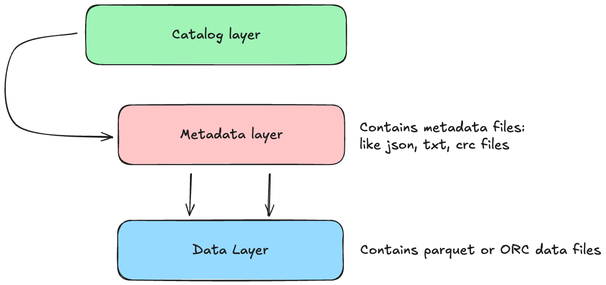
Catalog layer (eg. Glue Catalog, Hive Metastore,…) stores the current metadata pointer of the table
Metadata layer: it consists of a hierarchy of files (Json, crc and txt).

Metadata file: an authoritative JSON for the table at a point in time (contains table schema, partition config, and pointers to the current snapshot and previous snapshots). A new metadata file is created on every table update (commit).
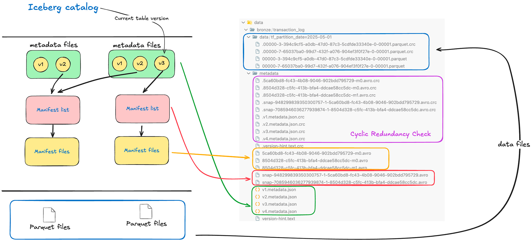
Manifest list: a file that lists all manifest files in a particular snapshot, along with partition summary stats for pruning. Each snapshot has at most one manifest list.
Manifest files: each manifest contains a list of data files (or delete files) belonging to that snapshot, along with row counts, file sizes, partition values, and min/max metrics for each column. Manifests allow query engines to quickly skip irrelevant files (partition pruning and data skipping) without loading all files.

Data files layer it contains the data files like Parquet or ORC files. The Data layer is the actual data files in storage (Parquet, ORC, Avro, etc.), which Iceberg treats as immutable datasets. If you perform an update or delete, Iceberg creates new files rather than mutating existing. Old data files remain untouched in older snapshots, ensuring time travel and isolation (more on this below). By separating the logical table from physical layout, Iceberg enables background optimizations (like file compaction) without interfering with running queries

The image below shows the mapping from Conceptual to Physical of Apache Iceberg

II. Features

Apache Iceberg has a large of features that enables Data Lake into Lake House.

ACID Guarantees and Transactions — When Writing in Iceberg (INSERT, UPDATE, DELETE, MERGE INTO) is a transactional commit that produces a new snapshot, and commits use atomic operations (usually an atomic swap of the metadata pointer) so that readers either see the entire commit or none of it. This means multiple users or engines can append or update data concurrently without corrupting table state. Iceberg ensures serializable isolation — readers will not see partial writes, and writers don’t interfere with each other’s uncommitted data. If a job fails mid-write, no half-finished data is visible; the last successful snapshot remains the table state. These ACID guarantees bring predictable consistency to data lakes,to transactions in a database. (Tip: Iceberg’s v2 table format introduced row-level UPDATE/DELETE/MERGE operations — ensure your table is using format-version 2 to have full ACID write support.)

Schema Evolution — Iceberg was built with the idea that schemas change over time. It supports in-place schema evolution that is full and flexible — you can add new columns, drop or rename columns, even change column types (with certain restrictions) without rewriting existing data files. These changes are stored as new metadata snapshots (it means that you don’t really change/modify the data files — it just changes the metadata files by creating new one), and old schema versions are tracked for consistency. Crucially, schema changes in Iceberg do not break queries on old data: Iceberg manages column IDs under the hood so that even if you rename a column, it still maps to the same field in the data files. For example, adding a new column will back-fill null values for existing rows (the data files aren’t immediately rewritten, just interpreted with nulls for the new field). This is a huge improvement over Apache Hive, where altering a schema often required painstaking migrations or had limitations. Iceberg’s approach ensures a smooth evolution of tables as requirements change, with all changes tracked in the table’s history.

Hidden Partitioning and Partition Evolution — Partitioning in data lakes is crucial for query performance, but Hive’s approach had several drawbacks. In Hive, partition columns are physically part of the data and must be manually managed (e.g., adding a partition column, and users must filter on it, and when user querying they have to know the partition column). If a user forgets to add the partition filter, Hive will scan all data. Iceberg introduces hidden partitioning feature, where partition values are derived from data by the table engine and stored in metadata – not exposed as separate columns. This means you can partition an Iceberg table by a transform (say, date(ts) or bucket(id, 100)), but queries can just filter on the original ts or id columns and Iceberg will know how to prune partitions automatically. Users don’t need to know the partition scheme to avoid full table scan. It also eliminates errors like wrong partition values – Iceberg always computes the partition values, so they’re consistent and correct.

Note: I didn’t use this feature (hidden partitioning), in my pipeline and my table I always define the partition columns and filter base on it.

Iceberg allows partition evolution, meaning you can change the partition strategy as your data grows, without rebuilding the table or losing historical data. Because queries don’t hardcode partition paths, you can, for example, start partitioning by day instead of month for new data going forward — in the same table. Iceberg tracks older and newer partition specs simultaneously and knows which files belong to which. This is done by versioning partition metadata, so a table can have multiple partition schemes over its lifetime. For instance, you might replace a partition field month(ts) with days(ts) as data volume increases, using a command like:

ALTER TABLE my_table 
REPLACE PARTITION FIELD month(ts) WITH days(ts);

Old files (partitioned by month) remain accessible and new files will use day partitions — but your queries don’t change at all and will correctly retrieve data across both schemes. This ability to evolve partitioning on the fly, without migrating data.

Time Travel — Every change in an Iceberg table creates an immutable snapshot. Because snapshots are retained (until explicitly expired), you can query or rollback to earlier table states — this is often called time travel (or you may hear about the table versioning). Iceberg assigns each snapshot a unique ID and timestamp. Using Spark SQL, you can easily query a past version of the table: for example, “show me the data as of yesterday”:

// Time travel by timestamp
SELECT * 
FROM prod.db.table TIMESTAMP AS OF '2025-05-15 00:00:00';

// Time travel to specific version
SELECT * 
FROM prod.db.table VERSION AS OF 10963874102873;

Pluggable Catalog & Multi-Engine Support — Iceberg is engine-agnostic by design. The catalog abstraction means Iceberg tables can be registered in a variety of metastore backends: Hive Metastore, AWS Glue, a simple Hadoop FS directory, a relational database, or a custom REST catalog (e.g., Netflix’s Azuretable or Nessie). The catalog handles table discovery and the atomic commit of the metadata pointer. This flexibility allows different processing engines to share the same table. A Spark job can write to an Iceberg table, and a Trino or Flink job can immediately read from it (and vice versa), because they all understand the Iceberg table format and consult the same catalog for metadata. In other words, Iceberg decouples the table’s state from any one engine. This is a big difference from Hive, where the Hive metastore was mainly accessed by Hive or Spark, or from proprietary Lake house formats tied to specific platforms.

Note: Iceberg also plugins Duckdb. I am a lover of DuckDB

III. Hands-on

Setup environment

All Code, File and Configuration I have written down in my public repository, you can view and following in here.

In this post, I used Apache Spark version 3.5.0 + Iceberg 1.6.1 which written by Scala version 2.12.

We just need the Spark container, execute inside container and run the spark-submit command to run the Spark Job to Interact with data (Create, Update, Delete and some features on Iceberg through Spark SQL).

// see the docker-compose file to setup Spark environment
>> spark-kafka-docker-template/infrastructure/standalone/docker-compose-spark.yml

version: '3'
services:
  spark:
    image: jupyter/pyspark-notebook:spark-3.5.0
    container_name: spark-notebook
    ports:
      - 8888:8888 # this port for Jypyter notebook
      - 2718:2718
    environment:
      - INIT_DAEMON_STEP=setup_spark
      - PYTHONPATH=${PYTHONPATH}:/home/jovyan
    volumes:
    - ../../src:/home/jovyan
    - ../../project:/home/jovyan/project
    - ../../assets/jars:/home/jovyan/jars
    - ../../data:/data
    - ../../requirements.txt:/home/jovyan/requirements.txt
    - ../../geeksdata:/home/jovyan/geeksdata
    working_dir:
      /home/jovyan
    command: ["jupyter", "notebook", "--no-browser","--NotebookApp.token=''","--NotebookApp.password=''"]

networks:
  standalone_net:
    external: true

Initialize and up the Spark docker container. Execute this command in root folder, make sure you have already installed the Make

// Step 1: Up the docker container
make up-spark
// Behind the scense: >> docker-compose -f infrastructure/standalone/docker-compose-spark.yml up -d
docker exec -it spark-notebook bash

// Step 2: Exec into the container then run the spark-submit job to submit the pyspark code
make iceberg
// Behind the scense: >>  spark-submit --jars /home/jovyan/jars/org.apache.iceberg_iceberg-spark-runtime-3.5_2.12-1.6.1.jar  geeksdata/data_engineer/table_format/iceberg_hands_on.py

This section will work with a sample table called customer. The customer table includes 4 fields:

customer_id: BIGINT
name: string
email string
country string

which is partitioned by country, to fully demonstrate how Iceberg works and to showcase its core features.

1. Creating Iceberg Table

We will use Spark SQL and configurate Iceberg dependencies to run Spark SQL to interact. In Spark SQL, the CREATE TABLE command can create an Iceberg table if you specify the USING iceberg clause or use a pre-configured Iceberg catalog:

-- Create an Iceberg table (partitioned by country)
CREATE TABLE IF NOT EXISTS optimus.bronze.customers (
  customer_id BIGINT,
  name        STRING,
  email       STRING,
  country     STRING
)
USING iceberg
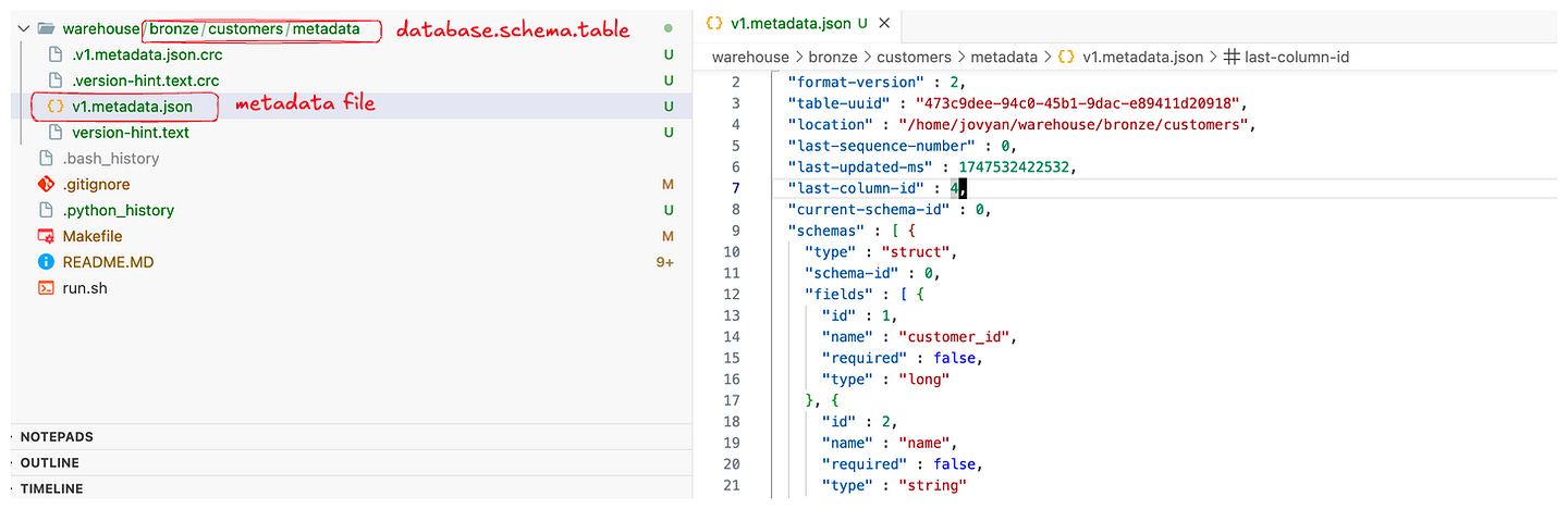
PARTITIONED BY (country);

Spark will create this table in the configured warehouse location (for example, a local /warehouse directory in the Docker container). The PARTITIONED BY (country) clause means Iceberg will partition data by country. Note that with Iceberg, the partition column country is part of the table schema (unlike Hive where partition columns could be separate). Iceberg will automatically manage the partition values under the hood. At this point, no data is in the table yet – but a metadata directory for customers is created, containing an metadata.json file (table definition) and ready to track snapshots.

Tip: You can verify the table exists by running a simple SELECT * (it will be empty) or by checking the metadata. For example, SELECT * FROM customers.history; would show an initial entry for table creation. The Iceberg catalog also tracks table properties like the format version (default is v2, which we need for upserts/deletes). If something isn’t working, make sure the table was indeed created as an Iceberg table (the USING iceberg clause or proper catalog prefix is crucial).

2. Insert into Iceberg table and Do some queries

We can use Spark’s standard SQL INSERT INTO with VALUES to add a few rows:

-- Insert some sample records into the Iceberg table
INSERT INTO optimus.bronze.customers VALUES 
  (1, 'Alice', 'alice@example.com', 'US'),
  (2, 'Bob',   'bob@example.com',   'CA'),
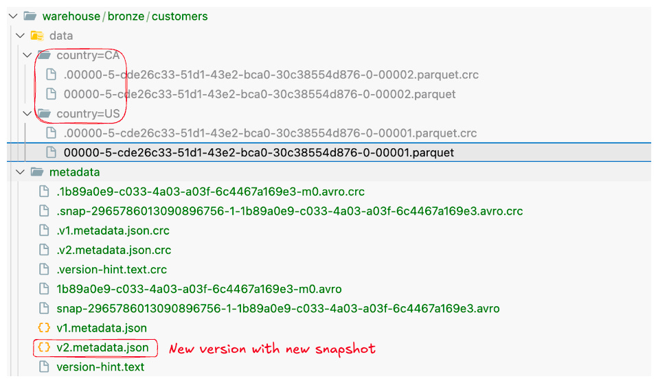
  (3, 'Carlos','carlos@example.com','US');

Iceberg will write these rows into one or more data files (Parquet by default). Because we only inserted a few records, likely all three went into a single small Parquet file in the country=US and country=CA partition folders (two partitions in this case). We can run a query to confirm the data was inserted:

SELECT customer_id, name, country 
FROM optimus.bronze.customers;

Behind the scenes, after this insert Iceberg created New Snapshot for the table. We can already explore what Iceberg is tracking in metadata.

3. Inspecting Table Metadata (Snapshots, Manifests, etc.)

One of the powerful aspects of Iceberg is the rich metadata it maintains. Iceberg exposes this via metadata tables that you can query with SQL. These are accessed by appending a special name to the table, like customers.history, customers.snapshots, customers.files, etc. Let’s take a look at a few:

Table History: shows a log of snapshots (by timestamp and snapshot ID).
Snapshots: detailed snapshot info, including operation (append, replace, etc), manifest list file, record count, etc.
Files: lists the data files in the current snapshot (with their partition values and stats).

Select history of table:

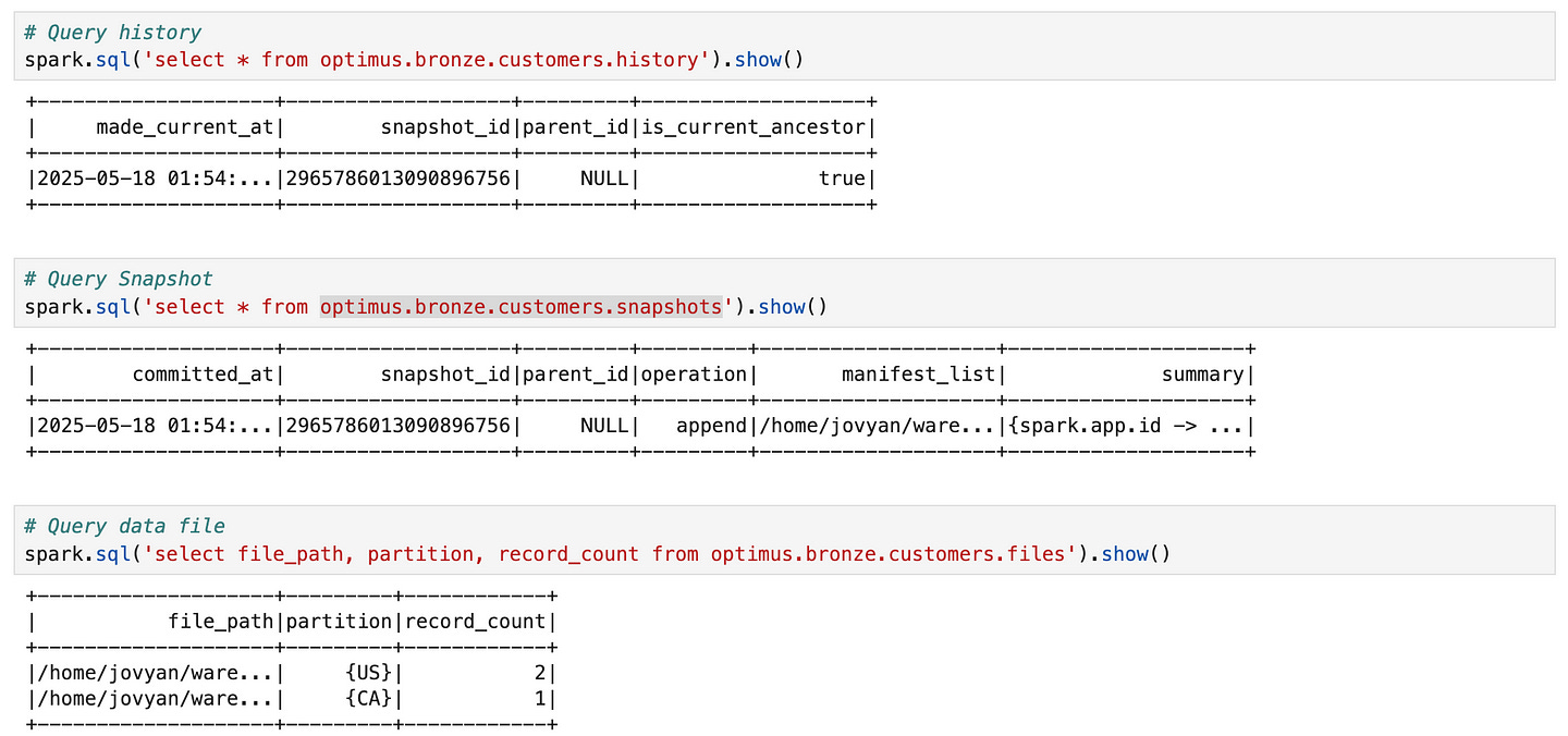
SELECT * FROM optimus.bronze.customers.history;

+--------------------+-------------------+---------+-------------------+
|     made_current_at|        snapshot_id|parent_id|is_current_ancestor|
+--------------------+-------------------+---------+-------------------+
|2025-05-18 01:54:...|2965786013090896756|     NULL|               true|
+--------------------+-------------------+---------+-------------------+

Here we see the timestamp of the commit and the snapshot ID (a big long number). parent_id is NULL because this was the first snapshot. If we query customers.snapshots, we’ll get one row with more details about Snapshot 1, for example (simplified):

SELECT * FROM optimus.bronze.customers.snapshots;

+--------------------+-------------------+---------+---------+--------------------+--------------------+
|        committed_at|        snapshot_id|parent_id|operation|       manifest_list|             summary|
+--------------------+-------------------+---------+---------+--------------------+--------------------+
|2025-05-18 01:54:...|2965786013090896756|     NULL|   append|/home/jovyan/ware...|{spark.app.id -> ...|
+--------------------+-------------------+---------+---------+--------------------+--------------------+

(The manifest_list is a file that lists the manifest(s) for this snapshot). We can also inspect the current data files via:

SELECT file_path, partition, record_count 
FROM optimus.bronze.customers.files;

+--------------------+---------+------------+
|           file_path|partition|record_count|
+--------------------+---------+------------+
|/home/jovyan/ware...|     {US}|           2|
|/home/jovyan/ware...|     {CA}|           1|
+--------------------+---------+------------+

This tells us two Parquet data files exist: one for country=US (with 2 records) and one for country=CA (with 1 record). Iceberg’s hidden partitioning is evident – we didn’t include country='US' in our query, but Iceberg still stored the data in partition folders and knows the partition value for each file. Any query filtering on country will only read the relevant files, without us having to specify a partition filter.

Also note the metadata folder for the table (not directly shown in the query above). If you list the warehouse/customers/metadata directory, you’d see files like v1.metadata.json, 9182716-...-snap.json (manifest list), and perhaps a manifest .avro file. The Iceberg catalog (e.g., Hive or Hadoop catalog) keeps a pointer to the latest metadata.json. This design allows us to time travel and track changes as we’ll see.

So far, we have a table with one snapshot (an append). Let’s perform some updates to see Iceberg’s ACID capabilities.

Let’s see what I did : ) You can see in my notebook file

4. Do Upsert and Verifying the correctness

A common scenario is needing to update some records and insert new ones — often termed upsert (update + insert). With Iceberg in Spark, we can do this in a single atomic operation using MERGE INTO (which is similar to SQL MERGE). Spark’s MERGE will handle matching rows and apply updates or inserts accordingly.

Suppose Alice’s email changed and we have a new customer Diana to add. We can perform an upsert like so:

MERGE INTO optimus.bronze.customers t
USING (
  SELECT 1 AS customer_id, 'Alice' AS name, 'alice@newdomain.com' AS email, 'US' AS country  -- updated Alice
  UNION ALL
  SELECT 4, 'Diana', 'diana@example.com', 'UK'                                              -- new customer
) s
ON t.customer_id = s.customer_id
WHEN MATCHED THEN 
  UPDATE SET *
WHEN NOT MATCHED THEN 
  INSERT *;

Let’s break down what this does. We created an inlined dataset s with two rows: one for customer_id=1 (Alice’s new info) and one for customer_id=4 (Diana). The MERGE compares s to the target table t on the customer_id key. For ID 1, which matches an existing row, it updates all columns (UPDATE SET * means set every column to the values from s). For ID 4, which is not in customers, the “not matched” clause inserts the new row. This entire merge executes as one transaction – Iceberg will apply row-level updates and inserts in a single snapshot commit.

After running the MERGE, we should verify the table state:

SELECT customer_id, name, email, country FROM optimus.bronze.customers;

+-----------+------+-------------------+-------+
|customer_id|  name|              email|country|
+-----------+------+-------------------+-------+
|          2|   Bob|    bob@example.com|     CA|
|          4| Diana|  diana@example.com|     UK|
|          1| Alice|alice@newdomain.com|     US|
|          3|Carlos| carlos@example.com|     US|
+-----------+------+-------------------+-------+

We see that Alice’s email was updated, Bob and Carlos remain unchanged, and Diana was added. Importantly, this happened without any downtime or intermediate inconsistency — any reader querying the customers table will either see the old data (before commit) or the fully updated data (after commit), never a partial update. Iceberg accomplished this by writing out new data files for the modified partitions under a new snapshot (let’s call it Snapshot 2) and atomically switching the table’s pointer to that snapshot when the MERGE committed. The old snapshot (Snapshot 1) is still preserved in metadata.

We can confirm the new snapshot was created by checking the snapshots again:

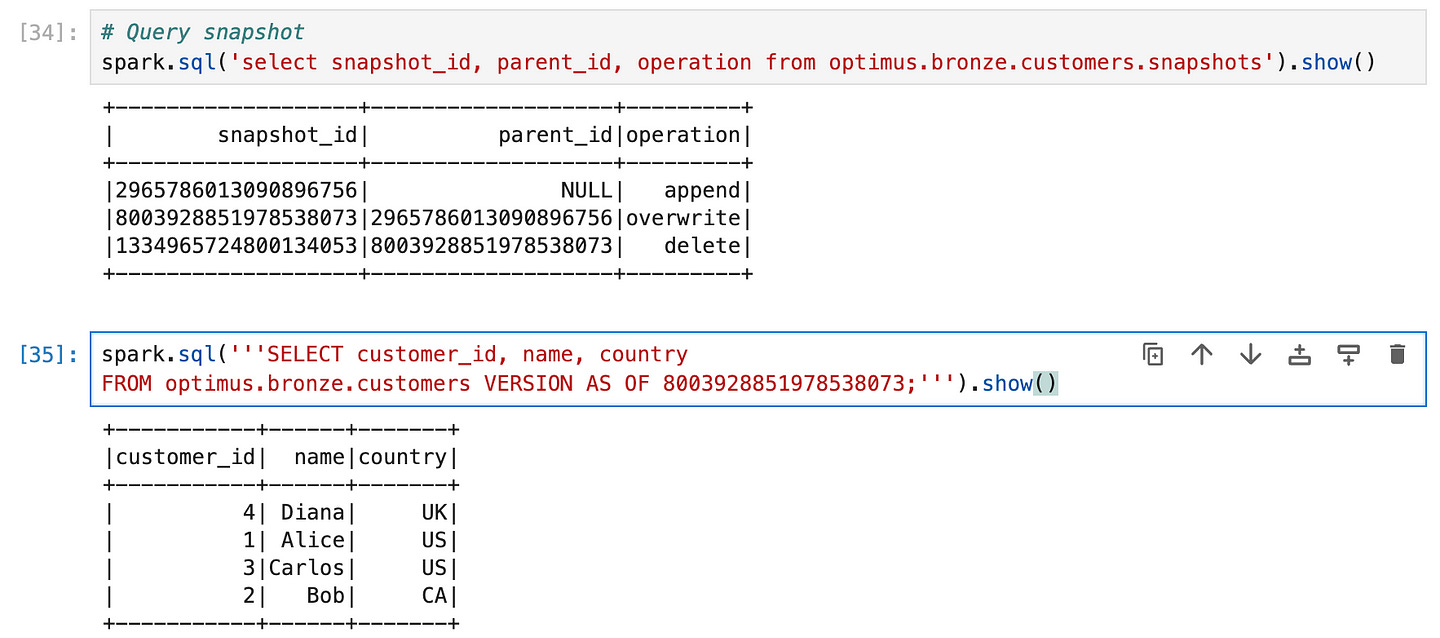
SELECT snapshot_id, parent_id, operation FROM optimus.bronze.customers.snapshots;

+-------------------+-------------------+---------+
|        snapshot_id|          parent_id|operation|
+-------------------+-------------------+---------+
|2965786013090896756|               NULL|   append|
|8003928851978538073|2965786013090896756|overwrite|
+-------------------+-------------------+---------+

The second entry (with a later timestamp) indicates a merge operation was performed, built on top of the first snapshot (parent_id points to the previous snapshot) — meaning Iceberg only updated the differences rather than rewriting everything. If we query customers.snapshots now, we’d see Snapshot 2 with operation replace or overwrite (depending on how Iceberg recorded the MERGE) and the updated manifest list.

5. Row-Level Deletes

Just as we updated and inserted, we can also delete rows with Iceberg. Spark SQL allows standard DELETE FROM statements on Iceberg tables. Let’s say Bob (customer_id 2) needs to be removed:

DELETE FROM customers 
WHERE customer_id = 2;

Iceberg will create yet another snapshot (Snapshot 3) for this delete operation. Under the hood, it doesn’t immediately wipe out Bob’s data file. Instead, Iceberg will rewrite the file that contained Bob, excluding his row (this is again copy-on-write deletion). In our case, Bob was in the country=CA partition in a file with just his record – Iceberg may optimize this as a metadata delete if the entire partition or file is removed. Often, if you delete all rows of a partition, Iceberg will simply drop that partition’s file from the snapshot (a metadata-only operation). Otherwise, it creates a new file for that partition without the deleted rows. Either way, Snapshot 3 will not include Bob’s record, but older snapshots still have it.

If we query the current table now:

SELECT customer_id, name, country FROM customers;

We’d get Alice, Carlos, and Diana — Bob is gone. The history table will have a third entry for the delete operation. And if needed, we can verify Bob is truly gone in current data:

SELECT * FROM customers WHERE customer_id = 2;

(no results). However — and here’s where Iceberg shines — Bob’s data is not lost. It’s still present in Snapshot 2 (and 1). We could time travel to see it, which we’ll do next. This soft-delete approach ensures that if a deletion was a mistake or if you need Bob’s record for an audit, you can retrieve it from the table’s past.

(Note: Iceberg also supports row-level delete files (called position deletes) in format v2.

6. Time Travel Queries (Querying Historical Data)

Now that we have multiple snapshots, let’s demonstrate time travel. Imagine we want to see the table as it was before Bob was deleted (i.e. after the upsert but before the delete). We can use the VERSION AS OF clause with the snapshot ID from Snapshot 2 to do that. First, find the snapshot ID for the state after the merge/upsert. We saw in the history that snapshot_id was, say, 8003928851978538073 for the merge. We’ll use that:

SELECT customer_id, name, country 
FROM optimus.bronze.customers VERSION AS OF 8003928851978538073;

+-----------+------+-------+
|customer_id|  name|country|
+-----------+------+-------+
|          4| Diana|     UK|
|          1| Alice|     US|
|          3|Carlos|     US|
|          2|   Bob|     CA|
+-----------+------+-------+

7. Compacting Small Files (Optimizing the Table)

Over time, especially with many small writes or merges, a table can accumulate lots of small data files. Too many files can degrade read performance (each file has overhead) and increase metadata size. Iceberg provides a way to compact small files into larger ones. This is done via the rewrite_data_files action/procedure. Using Spark SQL, we can invoke it as:

CALL optmius.system.rewrite_data_files(
  table => 'default.customers',
  options => map('min-input-files', '2')
)

(The exact catalog prefix may differ; here we assume optimus is our Iceberg catalog and the table is bronze.customers. In some setups, it could be CALL optimus.system.rewrite_data_files('bronze.customers').)

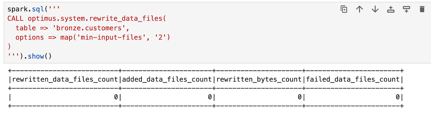
This procedure will scan the table for small files and combine them into fewer, larger files. We passed an option to only trigger if at least 2 small files can be merged. Iceberg’s compaction uses a bin-packing or sorting strategy to merge files without double-counting data. After running this, the table will commit a new snapshot (let’s say Snapshot 4) where some of the old data files are replaced by new, bigger files. The table’s data doesn’t change, but the layout is optimized.

We can verify the effect by checking customers.files again. For example, if previously we had separate files for Alice/Carlos vs Diana vs Bob’s partition, after compaction we might see fewer files. The manifest would also shrink. Compaction is a background optimization – queries can still run while it’s happening (if run via an asynchronous job), or if run inline as above, it’s a one-time operation that results in a new consistent state. By reducing small files, we reduce the metadata overhead and improve scan efficiency. This is one of those “table maintenance” tasks that Iceberg makes straightforward (others include expiring snapshots, removing orphan files, etc., which can be done with similar CALL procedures). In traditional lakes, compaction was a manual or MapReduce job;

Tip: It’s good practice to periodically compact especially if you use streaming or frequent small batch writes. Also, remember to expire old snapshots if you no longer need to time travel far back, as old snapshots keep old files alive. For example, CALL ... expire_snapshots(older_than => '2025-01-01') would remove snapshots before 2025 and their data files (if no longer referenced). This keeps storage usage in check.

Apache Iceberg is a powerful addition to the data engineer’s toolkit, offering the governance of a data warehouse on the flexibility of a data lake. We’ve seen how its architecture (table format, metadata layers) enables features like ACID transactions, time travel, and evolution of schema/partitions with ease. By trying these operations hands-on in Spark, you can appreciate the simplicity: no custom workflows or manual file management was needed — Iceberg handled it all under the hood. As you move from this 101 into real-world applications, you’ll find that Iceberg integrates with streaming jobs, batch ETLs, and interactive SQL engines, unlocking a truly unified data lakehouse experience. Happy data engineering with Geeksdata :D

GeeksData

Discussion about this post

Ready for more?